Neural Network is a buzzword being thrown around every page of every tech magazines. What really are they ? Contrary to popular belief God didn’t make them in six days. They have been around (or at least the concept of them) since the 40s when Donald O. Hebb, Fellow of the Royal Society proposed Hebbian Learning.
This was further improved when Frank Rosenblatt, built the “Mark I Perceptron” (Tony Stark inspiration ?) a mechanical equivalent capable of weight updates through electric motors.
These models ignored through the ages were thrown in a frenzy with the inception of GPU and massive albeit cheap computing power, which led to a Machine Learning boom.
The Lego Blocks: Neurons
The basic units of these “Neural Nets” are neurons. A single neuron is capable of computing a simple function, when these simple functions are stacked together they can represent complex functions, just like Legos.
A single neuron contains a weight, capable of taking a bunch of inputs and applying the weight to the inputs. This then passes through an appropriate activation function, which is the output of a single neuron.
It maybe represented as:
where $x_1, x_2, x_3, …x_n$ are the inputs, $w_i$ are the learned weight of the neuron and $g(x)$ is the activation function of the neuron.
The Quest for the Holy Grail: The Neural Nets
Now that you know so well about the basic building blocks of the neural nets let’s jump right into making one from scratch. We’ll use the Python library numpy (yep… just that) to make the network. But before that we’ll need data to make the Neural Net learn from. Let’s use the Anderson’s Iris data set made available by the UCI Machine Learning Repository. The dataset is in a format similar to the following:
| F0 | F1 | F2 | F3 | Y |
|---|---|---|---|---|
| 5.1 | 3.5 | 1.4 | 0.2 | 0 |
| 4.9 | 3.0 | 1.4 | 0.2 | 0 |
| 4.7 | 3.2 | 1.3 | 0.2 | 0 |
| 4.6 | 3.1 | 1.5 | 0.2 | 0 |
| 5.0 | 3.6 | 1.4 | 0.2 | 0 |
| … | … | … | … | … |
The F0-F3 are the features, whereas the 0-2 denotes the classes. The Iris dataset contains 3 classes, if your dataset is not in numerical format you can easily convert it with Python (or even a text editor). After you have downloaded the dataset and put it in a suitable directory let’s get started.
import numpy as np
import csv
The above lines imports the required libraries.
#Read Dataset
iris = open('iris.csv','r')
iris = csv.reader(iris,delimiter=',')
iris = np.array(list(iris))
Next we need to import our dataset and convert it into a numpy array, the statement np.array(list(iris)) does just that.
In the next step we’ll jumble the rows of the dataset a bit… this is to ensure that the distribution is uniform.
#shuffle dataset
np.random.shuffle(iris)
Since the last column is the label lets separate the features and labels. The first line of the following code accomplishes that. It is important to normalize (i.e. zero mean and standard deviation) our features; this ensures that the algorithm learns smoothly, here’s a great article by Sebastian Raschka detailing Feature Scaling and Normalization.
#all columns excluding the last is a feature last column is the label
features = iris[:,:-1]
features = (features - features.mean())/features.std()
In the above equation for neurons we have a term $b$, this is the bias term; it is necessary for times when the class labels are independent of the features. We add the bias as a column of 1 to the feature vector. It can be kept separate too.
#make a row sized vectors of 1
biasPad = np.ones((features.shape[0],1), dtype=features.dtype)
#pad 1s on the right side of each feature vector
features = np.concatenate((features,biasPad), axis=1)
Now lets make a final change to the representation, we’ll need the class labels in a One-Hot encoded format, we’ll use the following numpy trick to achieve that.
#create a one hot matrix repesentation of the labels
label = np.array(iris[:,-1],dtype=int).reshape(-1)
label = np.eye(3)[label]
Now that our features and labels are ready lets split ‘em up into training and testing set. An 80:20 training-to-testing set is the norm for small datasets.
#split training and testing set 0.8 split
M = features.shape[0]
splitIdx = int(0.8*M)
XTest = features[splitIdx:,:]
XTrain = features[:splitIdx,:]

YTest = label[splitIdx:,:]
YTrain = label[:splitIdx,:]
Let’s Stack ‘em Up: The Neuron Layers
Remember those simple neuron units capable of computing simple functions, let’s stack them into layers and put a couple of those layers together. This enables the network of neurons to compute complex functions as we have discussed earlier. Ours is gonna be a simple 3 layered network with a single hidden layer. The sizes of the hidden layer is a hyperparameter and you’ll have to iterate through a couple of models to get something that works out. Here we’ll keep the hidden layer size hiddenCount the same size as the input layer. We’ll also initialize the activation of the neural layers ai,ah and ao.
#neurons
#no of input neurons is equal to size of feature vector
inputCount = features.shape[1]
#basic case
hiddenCount = inputCount
#3 class classification thus 3 neurons
outputCount = 3

#activations for each layer of neurons
ai = np.ones((inputCount,1))
ah = np.ones((hiddenCount,1))
ao = np.ones((outputCount,1))
The Learnable Parameters: Weights
The weights are the parameters our neural network will actually learn. A matrix is a natural way to denote the fully connected layers of the neural network. We need to initialize our weights from a uniform distribution this is done to ensure that the network break symmetry by calculating different signals, else it’ll continue doing the same calculations. (Try it for yourself !!!). Here we use a initialization stratergy known as He Initialization proposed in the paper by He, Kaiming, et al. This stratergy is used so that the weights are not too large or too small which tends to cause problems of Exploding or Vanishing gradients while training; here’s a article by Imanol Schlag exploring the topic.
#neuron weights
#for each neuron in hidden layer calculate weights from ith input neuron
wih = np.random.rand(inputCount, hiddenCount)*np.sqrt(2./inputCount)
#for each neuron in output layer calculate weights from ith hidden neuron
who = np.random.rand(hiddenCount, outputCount)*np.sqrt(2./hiddenCount)
We’ll use a Gradient Decent Optimizer known as Momentum. This will ensure our network learns faster. More on this later but let’s initialize the required matrices here.
#Update Arrays for momentum updates
cih = np.zeros((inputCount, hiddenCount))
cho = np.zeros((hiddenCount, outputCount))
The Feed Forward Function

Who doesn’t love cat videos ? Source: GIPHY
The feedFwd() function calculates a single forward pass for the neural network. This function returns the calculated output of the neural network. The argument featureMat can have any number of rows but the number of columns should be the size of the input layer that is number of features + 1 for bias. We’ll use tanh as an activation function. The first output will be calculated using random weights so the results will be as wrong as the flat earth believers; but our Network will start learning soon.
The following lines of Python code calculates the equation given below:
where $X$ is the training examples and $W_{ih}$ is the weight matrix between input layer and the hidden layer. Please see we have added an extra column for the bias term else the first equation would have been
But we’ve already taken care of that, so, no worries!
#function for feed forward calc
def feedFwd(featureMat):
    global ai,ah,ao,wih,who
    #input activations
    ai = featureMat

    '''hidden activations
    vectorized matrix multiply'''
    ah = np.dot(ai,wih)
    #vectorized activation function
    ah = np.tanh(ah)

    '''output activations'''
    ao = np.dot(ah, who)
    #vectorized activation function
    ao = np.tanh(ao)

    return ao
The Learning Step: BackPropagation

We have to go back. Source: GIPHY
Back Propagation is the step that allows the neural network to learn from the data. It uses a method known as Gradient Descent. Gradient Descent is used to find the optimal solution to a problem by minimizing a cost function. In our network we have used Quadratic Error as a cost function, it is written as:
where $\widehat{y_i}$ and $y_i$ are the ith ground truth label and the ith calculated label respectively. Our network minimizes this cost function by moving towards the minima of the function space. Intutively think of it as going down a hill while being blind-folded. Your best bet to go downhill is moving to the immediate lowest spot you can step on (no cliff jokes here !). Your step size is analogous to learning rate (and then the Lord said let there be another hyperparameter) in gradient descent. If you take really small steps it’ll take you a lot of time to reach the bottom, on the other hand if you have record breaking long legs… and I mean Looong, you will never comfortably reach the bottom.
Mathematically this going downhill can be acheived by calculus wizardy, or more technically; calculating the gradient of the error function and tweaking our parameters accordingly. The equation that represents the backpropagation is given as follows:
Then the weight updates are carried out as:
where $\alpha$ is the learning rate.
The term $(1 - A_h ^2)$ in the third equation is the result of using $tanh(x)$ as our activation function whose derivative is $1 - tanh(x)^2$. If you are curious as to how these equation are derived read this excellent article by Brian Dolhansky on BackPropagation.
Momentum Optimzations
Remember that cih and cho defined for momentum updates? Here’s where it really shines. Considering our going downhill example; momentum works, if you imagine yourself having a bit of speed while going down, this will disable you from making drastic direction changes while you descend. The same principle intutively applies to Momentum upgrades of the weights. Mathematically it is based on the principal of running average of the weight updates, and can be represented as:
For brevity we use $\beta.\theta_{t}$ only, which works fine.
#function for backpropagation
def backProp(X,label,output,N,batchSize=1,beta=0.0009):
    '''N: learning rate'''
    global ai,ah,ao,wih,who,cih,cho

    delOut = output - label
    dwho = np.dot(ah.T,delOut)/batchSize

    delHidden = np.dot(delOut,who.T)*(1.0 - ah**2)
    dwih = np.dot(X.T,delHidden)/batchSize


    '''weight updates'''
    who -= N*dwho + beta*cho
    cho[:] = dwho

    wih -= N*dwih + beta*cih
    cih[:] = dwih
The Training Function
Now let’s write the function for training our neural network. Our neural network is trained in the following method first the ouput values and it’s corresponding error from a feed forward pass is calculated. The backward pass is used to tweak the weights to reduce this error. Iteratively doing this for a number of epoch lets our neural network learn from the data.
Our dataset is quite small about 120 data in the training set, for large datasets with over million of cases, the operations overflows the memory capacity. Thus Gradient Descent can be done in three diffrent flavours, the backward pass can be calculated on:
- Vanilla Gradient Descent: All training data at once.
- Mini Batch Gradient Descent: A few of the data at once, generally in the powers of 2 like 16, 32, 64.
- Stochastic Gradient Descent: One training example at once.
The train function lets us use all three by using the parameter batchSize, when set to $M$, the size of the dataset; it runs Vanilla Gradient Descent. Setting the batch size to $1$ trains the network using a Stochastic Gradient Descent, any other values and we can train the network using Mini Batch gradient Descent. Here is a great article by Andy Thomas at adventuresinmachinelearning.com dicussing all three types of Gradient Descent in detail.
While training we also decay the learning rate and the momentum parameter every few iteration this ensures that the learning process will not overshoot the optima. This weight decay can be written as:
where $\eta$ is the decay rate. This method is known as Inverse Time Decay.
def train(X,Y,iteration=1000,learningRate=0.001,batchSize=1,beta=0.099,decayRate=0.01):
    errorTimeline = []

    #train it for iteration number of epoch
    for epoch in xrange(iteration):

        #for each mini batch
        for i in xrange(0,X.shape[0],batchSize):
            #split the dataset into mini batches
            batchSplit = min(i+batchSize,X.shape[0])
            XminiBatch = X[i:batchSplit,:]
            YminiBatch = Y[i:batchSplit,:]

            #calculate a forwasd pass through the network
            output = feedFwd(XminiBatch)

            #calculate Quadratic error
            error = 0.5*np.sum((YminiBatch-output)**2)/batchSize
            #print error

            #backprop and update weights
            backProp(XminiBatch,YminiBatch,output,learningRate,batchSize,beta)

        #after every 50 iteration decrease momentum and learning rate
        #decreasing momentum helps reduce the chances of overshooting a convergence point
        if epoch%50 == 0 and epoch > 0:
            learningRate *= 1./(1. + (decayRate * epoch))
            beta *= 1./(1. + (decayRate * epoch))
            #Store error for ploting graph
            errorTimeline.append(error)
            print 'Epoch :',epoch,', Error :',error

    return errorTimeline
Let’s Train the Network
Now let’s call the above functions with suitable hyperparameters to train our network on the Iris Dataset. To do this we just need the following lines:
#Work it, make it, do it,
#Makes us harder, better, faster, stronger!
learningRate = 0.0001
beta = 0.099

errorTimeline = train(XTrain,YTrain,2000,learningRate,M,beta)
Thus our network is trained for 2000 epoch with a learning rate of 0.0001 and using Vanilla Gradient Descent. If we plot the graph of training errors we get the following graph. We can observe that the values doled out by our network are more accurate as training continues.
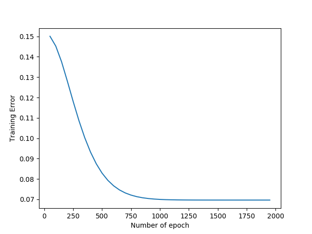
Training Error Plot
Moment of Truth: Testing Our Network
Now that our network is trained let’s use our testing set to test how good our network is. Just a reminder that the testing set consists of data our network has never seen before. We pass the test set through a forward pass of the network with the learned weights. The predOutput saves the returned output, we then compare this with the ground truth labels YTest.
#How tough are ya ?
#get output for test features
predOutput = feedFwd(XTest)
#vectorised count compare the indices of output and labels along rows
#add to count if they are same
count = np.sum(np.argmax(predOutput,axis=1) == np.argmax(YTest,axis=1))
#print accuracy
print 'Accuracy : ',(float(count)/float(YTest.shape[0]))
We see that the network reaches accuracy of over 97% for the testing set. Thus we’ve succesfully made a neural network that accurately identifies Iris plant species… and that too from scratch! Neural Network are versatile devices capable of achieving unbelievable tasks with shocking accuracy. Try experimenting with diffrent datasets and share your experience in the comments below. You can find the complete code here. Share your love by refering this article. Stay Tuned for more articles like this!!!