Convolution Neural Network in Keras for Digit Recognition!

Neural Networks are incredible and robust tools with wide range of application. Their use in computer vision is wide spread and well-studied. While the concept of Convolutional Neural Network have been around, the first break-through work with CovNets were done by Yann LeCun back in 1998 for AT&T Labs-Research which were widely used to recognize hand-written digits on a bank cheque. These networks took the spolight in 2012 when AlexNet won the ImageNet Large Scale Visual Recognition Challenge. Today availabity of cheap GPU, cloud instances amd robust machine learning frameworks like TensorFlow and Keras enables us to train these complex networks with ease.
This post explores how to build a CovNet for recognizing hand-written digits using Keras and the MNIST dataset by LeCun. Keras provides a handy API to build and test Neural Networks. It uses TensorFlow or Theano as a backend to give a simpler control over our networks. For this experiment we’ll use TensorFlow as our backend, so you need to have Python, TensorFlow and Keras installed on your machines or cloud instances.

It’s All about the Data

Neural Network needs a lot of data to figure out the patterns and make prediction. So to train our hand-written digit recognizer we have to give it abundance of hand-written digits to look at. MNIST dataset is perfect for our pursposes. It provides 60,000 size normalized and centered images for training. And an additional 10,000 images for testing !

Let’s get started!

from keras.datasets import mnist
from keras.preprocessing.image import ImageDataGenerator
from keras.models import Sequential
from keras.layers import Dense, Dropout, Flatten, Conv2D, MaxPooling2D
import keras

We need to import the required APIs from Keras. Moreover Keras provides keras.datasets which can be used to easily download and load a few selected datasets. Luckily for us MNIST is one of them. The rest of the import will be useful to define our neural network and its attributes.
So let’s go ahead define a few variables and load our dataset.

batch_size = 64
num_classes = 10
epochs = 30
img_h, img_w = 28, 28   # image dimensions

# load the data
(X_train, Y_train), (X_test, Y_test) = mnist.load_data()

What our Dataset looks like
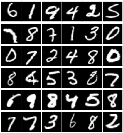
MNIST Image Samples

Each image of MNIST dataset is 28x28 in dimensions. Next we need to reshape our data to (img_h, img_w, 1) since TensorFlow uses NHWC (where N is number of images, H is Height, W is Width, C is number of channels) order also know as channel last order to represent the images.
We want to do all our operations in single point precision so we convert our data to 32-bit floating point and standardize it. Since pixel values ranges from 0 to 255 we can easily achieve standardization by X_train /= 255. The last step is One-Hot Encoding the class labels for which keras provides a handy function to_categorical.

X_train =  X_train.reshape( X_train.shape[0], img_h, img_w, 1)
%replace with -1
X_test = X_test.reshape(X_test.shape[0], img_h, img_w, 1)

X_train =  X_train.astype('float32')
X_test = X_test.astype('float32')
X_train /= 255
X_test /= 255

#convert to one hot encodings
Y_train = keras.utils.to_categorical(y_train, num_classes)
Y_test = keras.utils.to_categorical(y_test, num_classes)

Convolutional Layers: The Eye to the Brain

The Lego blocks of a CovNet is based upon the principle of matrix convolution.
Given matrix $M$ of size $(x,y)$ and kernel $N$ of size $(k,l)$ convolution operation can be represented as:

$(M \ast N)_{ij} = \sum_{p = 1}^{k - 1} \sum_{q = 0}^{l - 1} M(i-p, j-q)N(p,q)$

Intutively this is sliding a kernel $N$ over our image and taking a summation of the entrywise product of the overlapping regions. Let’s take an example and see how it works. Let $A$ be a 4x4 matrix.

$A = \begin{bmatrix} 10 & 5 & 8 & 11\\ 9 & 6 & 12 & 3\\ 2 & 1 & 4 & 3\\ 13 & 4 & 7 & 6 \end{bmatrix}$

And $B$ be our 2x2 kernel.

$B = \begin{bmatrix} 1 & 0\\ 0 & -1 \end{bmatrix}$

The convolution operation $A \ast B = C$ goes as follows:

$C_{1,1} = 10.1 + 5.0 + 9.0 + 6.(-1)\\ C_{1,2} = 5.1 + 8.0 + 6.0 + 12.(-1)$

and so on. Finally giving the results $C$ as

$A \ast B = \begin{bmatrix} 10 & 5 & 8 & 11\\ 9 & 6 & 12 & 3\\ 2 & 1 & 4 & 3\\ 13 & 4 & 7 & 6 \end{bmatrix} \ast \begin{bmatrix} 1 & 0\\ 0 & -1 \end{bmatrix} \\ = \begin{bmatrix} 4 & -7 & 5\\ 8 & 2 & 9\\ -2 & -6 & -2 \end{bmatrix}$

As you may have observed our resultant matrix $C$ is of size $3 \times 3$. This is a property of Convolutions, for image $I$ of size $W \times H$ and kernel $K$ of size $F \times F$ the activation after a convolutional layer will be $(H-F)/S+1 \times (W-F)/S+1$. Each convolutional neurons activates on data in its own receptive fields. That means conceptually the neurons learns filters that activate when the see some specific type of feature. In the initial layer the network learns simple features like diffrent orientation of lines, as we go deeper we see increasingly complex features learned by the network. This esentially does away with the need of designing hand-crafted features for computer vision tasks.
Now let’s start building our neural net!

model = Sequential()
model.add(Conv2D(filters=32, kernel_size=(3, 3),
                 activation='relu',
                 input_shape=X_train.shape[1:]))
model.add(Conv2D(filters=64, kernel_size=(3, 3),
                 activation='relu'))

The Keras Sequential model API lets us define our network as stack of layers. Let’s stack them up with Convolutional layers. Keras’s layers API provides us with Conv2D that help us describe our Convolutional Layer. Our network starts with 2 Convolutional Layers. The first layers has 32 filters. Filters signify how many depth slices our Convolutional layer has. Each filters provides us with a 2D feature map, using 32 filters thus makes our feature map 32 layers deep. Convolutional Layers uses parameter sharing, that is the learned weight can be applied against the entire image to reduce the number of parameters, this also enables the CNN to activate for features regardless of its spatial locality. During the backpropagation pass the operation is a convolution, but with a spatially flipped filter, this has been discussed in detail in this excellent article by Jefkine Kafunah. As in Vanilla NeuralNet CNN also uses activation function, $ReLU$ activation has been seen to work best. It’s important to pass the input shape as a parameter in the first layer, Keras will calculate it for us in the succeeding layers.

Pooling Layers

Pooling layers are zero-parameter layers between two convolutional layers. These reduces the dimentionality by downsampling our parameters thus reducing overfitting and also ensuring spatial invariance. Max Pooling is the most commonly used pooling. Intuitively think of it as sliding a $k \times k$ kernel over the output of the Convolutional layers, and using the max element of the overlapping region. This reduces the height and width of the parameters while keeping the depth intact. Most commonly used size is 2x2 in size with a stride of 2, as larger size tends to lose too much information. During backpropagation the operation is as simple as transferring the gradient to the max input element.
Let’s see Pooling in action with an example. Let $A$ be our activation map, and we have a kernel of size $2 \times 2$ then the result of Max Pooling, $R$ is as follows:

$A = \begin{bmatrix} 10 & 5 & 8 & 11\\ 9 & 6 & 12 & 3\\ 2 & 1 & 4 & 3\\ 13 & 4 & 7 & 6 \end{bmatrix}\\ R = \begin{bmatrix} 10 & 12\\ 13 & 7 \end{bmatrix}$

So let’s add our remaining layers to our network!

model.add(MaxPooling2D(pool_size=(2, 2)))
model.add(Dropout(rate=0.25))
model.add(Conv2D(filters=128, kernel_size=(3, 3),
                 activation='relu'))
model.add(MaxPooling2D(pool_size=(2, 2)))
model.add(Dropout(rate=0.25))

MaxPooling2D lets us add pooling layers to our network. We’ll also add a Dropout layer after the Pooling Layer. Dropouts are simple but powerful reguralization techniques first studied by Srivastava et. al. in their 2014 paper that prevents the network from overfitting. In dropout we randomly set a few activations to zero, this forces the network to generalize on the data distribution, since it randomly looses activations. Keras’s Dropout makes it convenient to use the dropout layers which takes a parameter which is the rate of dropout. Our nework will have one more Convolutional Layer followed by a pooling layer and dropout.

The Fully Connected Layers

The last few layers of a CovNet is fully connected neural net. This has full connectivity over the previous layers. We’ll use a two layer network using Keras’s Dense Layers API. Since our network is still in 2D so we’ll need to flatten it before we can attach the Fully Connected Layers, this can be acheived with Flatten. So let’s add the final part of our CovNet.

model.add(Flatten())
model.add(Dense(units=128, activation='relu'))
model.add(Dropout(rate=0.5))
model.add(Dense(units=64, activation='relu'))
model.add(Dropout(rate=0.5))
model.add(Dense(units=num_classes, activation='softmax'))

So that’s our whole network capable of recognizing hand-written digits after training. We’ll compile the model using model API’s compile function. The compile function takes in a few parameters that describes the network’s hyperparameters. In our network we’ll use the Categorical Crossentropy loss. It is written as:

$L(y,\widehat{y}) = - \sum_n \sum_i y_i^{(n)} log \widehat{y}_i^{(n)}$

for the $i$-th class and $n$-th training example. This loss function helps us estimate how far our predictions are from the actual class labels.
In our network we’ll also use $Adam$ optimizer for Gradient Descent Optimzation and $Accuracy$ as our metric to measure performance.
So let’s go ahead and compile our model!

model.compile(loss=keras.losses.categorical_crossentropy,
              optimizer=keras.optimizers.Adam(),
              metrics=['accuracy'])

Now that our model is compiled you can use the model API’s summary function to view a detailed summary of our network as given below. Our network has 511,306 trainable parameters!

_________________________________________________________________
Layer (type)                 Output Shape              Param #   
=================================================================
conv2d_1 (Conv2D)            (None, 26, 26, 32)        320       
_________________________________________________________________
conv2d_2 (Conv2D)            (None, 24, 24, 64)        18496     
_________________________________________________________________
max_pooling2d_1 (MaxPooling2 (None, 12, 12, 64)        0         
_________________________________________________________________
dropout_1 (Dropout)          (None, 12, 12, 64)        0         
_________________________________________________________________
conv2d_3 (Conv2D)            (None, 10, 10, 128)       73856     
_________________________________________________________________
max_pooling2d_2 (MaxPooling2 (None, 5, 5, 128)         0         
_________________________________________________________________
dropout_2 (Dropout)          (None, 5, 5, 128)         0         
_________________________________________________________________
flatten_1 (Flatten)          (None, 3200)              0         
_________________________________________________________________
dense_1 (Dense)              (None, 128)               409728    
_________________________________________________________________
dropout_3 (Dropout)          (None, 128)               0         
_________________________________________________________________
dense_2 (Dense)              (None, 64)                8256      
_________________________________________________________________
dropout_4 (Dropout)          (None, 64)                0         
_________________________________________________________________
dense_3 (Dense)              (None, 10)                650       
=================================================================
Total params: 511,306
Trainable params: 511,306
Non-trainable params: 0
_________________________________________________________________

The only thing left to do now is training our very own CovNet. We’ll use the model API’s fit function to accomplish this. We’ll train our network for 30 epochs in batch sizes of 64. While training we’ll use our testing set to calculate validation loss and accuracy. So let’s code that up already!

model.fit(X_train, Y_train,
          batch_size=batch_size,
          epochs=epochs,
          verbose=1,
          validation_data=(x_test, y_test))

Training Plot
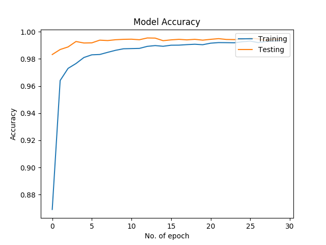
Training Accuracy and Loss Plot

In a standard laptop with nVidia GT940 video card this takes ~15 minutes to train. After we are done with training it’s the moment of truth, we’ll finally see how our model performs!

score = model.evaluate(X_test, Y_test, verbose=0)
print('Test loss:', score[0])
print('Test accuracy:', score[1])

We see that we are able to recognize hand-written digits with 99.33% accuracy! There you go, you have successfully built your own CovNet. One caveat of CovNets are that it takes long time to train on underpowered machines, good news is that you rarely have to train a CovNet from scratch, you can take a pre-trained CovNet and fine tune it to your dataset, thus eleminating long training times! We’ll explore this in a future article. Meanwhile try experimenting with your own datasets.
Live long and prosper!